Teacher Demonstration
Use the live model as a shared screen demonstration before students try their own predictions and observations.
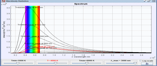
Explore Intro Page as an interactive EJS simulation for waves and optics.
Use the live model as a shared screen demonstration before students try their own predictions and observations.
Open the simulation, adjust the controls, and compare what changes on screen before answering the concept-check questions.
Which variable is held constant, which is changed, and how does particle motion explain the gas-law pattern?
Decide whether the comparison is isothermal, constant volume, or another controlled condition.
Adjust volume, temperature, or particle number while observing pressure or graph changes.
Use collision frequency and particle speed to explain the macroscopic result.
Check that the graph pattern and particle-level explanation agree.
Use this as a micro-macro bridge for gas laws. Students should not only quote PV = nRT; they should explain the observed pattern using collisions.
Ask: Why does pressure increase when volume decreases? What does temperature change do to particle speed? Which variable was controlled in your comparison?
Pair a graph reading with a particle explanation. This helps students move between symbolic gas laws and the kinetic model.
These questions are generated from the topic and the concept illustrated by the simulation. Use them after students have explored the model.
Correct first attempts build a streak and unlock higher point multipliers on this device.
1. What does an ideal-gas model connect?
2. If volume decreases while temperature is kept similar, what tends to happen to pressure?
3. What is the microscopic reason for gas pressure?
4. Why compare isothermal or controlled cases?
5. What evidence should students cite?
Anonymous activity counts show that this resource is being discovered and used.